Guest Post By Colin Banfield
29th September, 2011
Equivalents of Excel’s Percentile, Quartile, and Median functions are perhaps the most significant omissions in Denali’s DAX statistical function library. Quartile and Median are actually special cases of percentile, and in this post, we calculate these special cases. Some of the most insightful BI analysis involves the use of statistics, and PowerPivot provides an excellent environment for developing statistical measures. Perhaps percentile and its cohorts will be considered for inclusion in PowerPivot V3.
Percentile measures are not difficult to create in DAX, but the process is also not trivial. Adding to the complexity is the need to interpolate values if you want to duplicate the accuracy of Excel’s percentile functions. My approach to creating percentile measures in PowerPivot is as follows:
- Calculate the ascending rank of values in the dataset under exploration.
- Calculate the rank corresponding to required percentile. I use the formula n=P(N-1)/100+1, where n is the rank for a given percentile P, and N is the number of rows in the dataset. This formula provides the rank corresponding to Excel’s PERCENTILE or PERCENTILE.INC function. For a calculation equivalent to Excel’s PERCENTILE.EXC, the rank for a given percentile can be found by using the formula n=P(N+1)/100. In most cases, the rank calculated will not be an integer. Therefore, for a generalized solution, we must use the integer rank below and above the calculated value and interpolate. For example, the first formula in (1) calculates a rank of 11.25 for P=25 (25th percentile) and N=42. We must therefore interpolate between the dataset ranks of 11 and 12.
- Find the data values corresponding to the integer ranks derived from step 2. For convenience, let’s call these values PPercentileDown and PPercentileUp.
- Calculate the percentile using linear interpolation.
Let’s start with a simple dataset to illustrate the concepts. In figure 1, the original dataset is in the table on the left. The corresponding PowerPivot PivotTable is on the right.
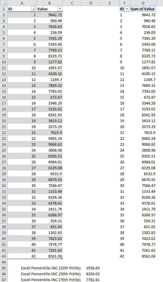
Figure 1- Original Dataset
Step 1 – Calculate the ascending rank of values in the dataset
Fortunately, the newly minted RANK function in Denali makes the calculation a lot easier than the rank formula we had to create in V1. The rank formula is simply:
=RANKX(ALL(Data),[Sum of Value],,1)
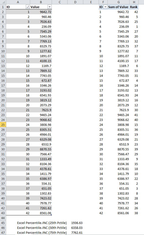
Figure 2 – Rank Measure
Step 2 – Calculate the rank corresponding to required percentile
We will first calculate the rank corresponding to the 25th percentile (inclusive) in the dataset. Recalling the formula n=P(N-1)/100+1, this translates into the following DAX formula:
=CALCULATE(
(COUNTROWS(Data)-1)*25/100+1,
ALL(Data)
)
In this case, the calculated rank is 11.25.
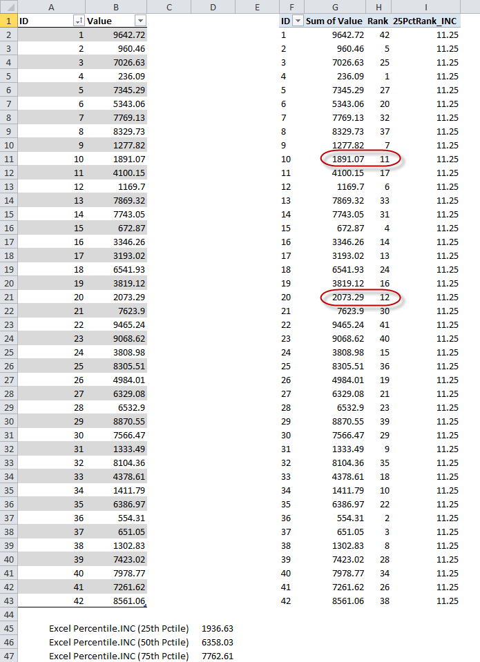
Figure 3 – Rank of 25th percentile
Step 3 – Find the data values corresponding to the integer ranks derived from step 2
Our 25th percentile value is somewhere between the values corresponding to the 11th and 12th rank, as shown in figure 3. We need formulas to extract these values as measures. The 25thPercentileDown formula is:
=MAXX(
FILTER(
ALL(Data),
[Rank] = ROUNDDOWN([25PctRank_INC],0)
),
[Sum of Value]
)
We are returning the Max of Sum of Value, filtered so that [Rank] is equal to the rank of the 25th percentile, rounded down to the nearest integer rank. In other words, we are filtering the table to return only values where [Rank] = 11. In the case of ties, there will be more than one value in the filtered table (all identical). This is the reason for using MAXX. However, MINX, or even AVERAGEX would calculate the same result.
For 25thPercentileUp, you may be inclined to use a similar formula, substituting the ROUNDDOWN function for ROUNDUP. However, in the event of ties for the 25th percentile, the filter will be incorrect. This is so because [Rank] will calculate the same rank for ties (11 in this case), and ROUNDUP([25PctRank_INC],0)will be = 12. We can get around the problem by filtering the table using the TOPN function instead:
=MAXX(
TOPN(
ROUNDUP([25PctRank_INC],0),
ALL(Data),
[Sum of Value],
1
),
[Sum of Value]
)
The formula simply finds the max of the top 12 values in the dataset (i.e. 11.25 rounded up to 12). The result is not affected by ties in the rank. Figure 4 shows the resultant measures.
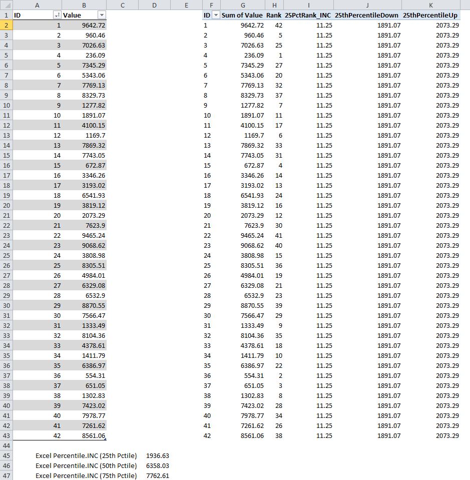
Figure 4 – Rankup and Rankdown
Step 4 – Calculate the percentile using linear interpolation
Now that we have the values between which we need to interpolate to find the actual percentile, we use these values in a simple interpolation formula:
=[25thPercentileDown]+([25thPercentileUp]-[25thPercentileDown])*([25PctRank_INC]-ROUNDDOWN([25PctRank_INC],0))
= 1891.07 + (2073.29-1891.07)*(11.25-11) = 1891.07 + 182.22*0.25 = 1936.63
In figure 5, I’ve completed the calculations for the 50th percentile and 75th percentile and removed intermediate formulas from the PivotTable.
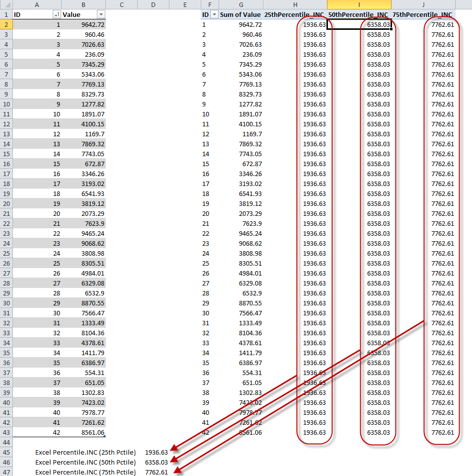
Figure 5 – Percentiles
Figure 5 illustrates that that values we calculated are identical to values calculated by using Excel’s PERCENTILE.INC function. Note that:
- The 25th percentile is also the first quartile
- The 50th percentile is the median (i.e. the same value returned by Excel’s MEDIAN function)
- The 75th percentile is also the third quartile
Alternative median calculation
If we need to calculate the median without regard for percentiles, we could use the following formula:
=IF(
MOD(
COUNTROWS(ALL(Data)),
2
)=0,
AVERAGEX(
TOPN(
2,
TOPN(
(COUNTROWS(ALL(Data))/2)+1,
ALL(Data),
[Sum of Value],
1
),
[Sum of Value]
),
[Sum of Value]
),
MAXX(
TOPN(
COUNTROWS(ALL(Data))/2,
ALL(Data),
[Sum of Value],
),
[Sum of Value]
)
)
Essentially, we want to return the value in the middle of the range, after sorting the range in ascending order. The calculation we use depends on whether there are an even or odd number of values in our dataset. The first part of the formula, MOD(COUNTROWS(ALL(Data)),2)=0, determines if the dataset has an even number of values. I would have preferred to use ISEVEN (and thus eliminate an extra function call), but alas, Excel’s ISEVEN and ISODD functions didn’t make it into DAX.
If the number of values is even, we need to get the top value in the first half of the dataset, plus the next higher value (because we have to average these two values to get the median). We accomplish this goal in the following part of the formula:
TOPN(
(COUNTROWS(ALL(Data))/2)+1,
ALL(Data),
[Sum of Value],
1
)
Based on our sample dataset, the preceding formula will return a table with values where ID=1 to ID=22. Next, we get the top 2 values from this new table (ID=21 and ID=22). To accomplish this task, we wrap another TOPN function around the new table and sort in descending order:
TOPN(
2,
TOPN(
(COUNTROWS(ALL(Data))/2)+1,
ALL(Data),
[Sum of Value],
1
),
[Sum of Value]
),
Finally, we average the two values:
AVERAGEX(
TOPN(
2,
TOPN(
(COUNTROWS(ALL(Data))/2)+1,
ALL(Data),
[Sum of Value],
1
),
[Sum of Value]
),
[Sum of Value]
),
If the number of values in the dataset is odd, we just return the middle number, using the formula in the final argument of IF:
MAXX(
TOPN(
COUNTROWS(ALL(Data))/2,
ALL(Data),
[Sum of Value],
),
[Sum of Value]
)
Note that TOPN rounds a number up or down arithmetically, if the first argument is a decimal value. Dividing an odd number by 2 will therefore always round the number to the next higher value.
Percentile INC vs. EXC
At the beginning of this post, I mentioned that to compute percentiles corresponding to Excel’s PERCENTILE.EXC, you use the formula n=P(N+1)/100 to get the rank for a given percentile. When, therefore, should you use one versus the other? The answer is similar to the use of STDEV.S/STDEV.P or VAR.S/VAR.P. PERCENTILE.EXC, which is a new function in Excel 2010, generally provides better results when we are using a sample from a larger dataset (where it’s unlikely that the sample would include the dataset’s zero and one-hundredth percentile values – and thus these percentiles are excluded). PERCENTILE.INC is better when we’re working with the entire dataset.
My rants of the day
Rant #1
I can’t help but end this post with a couple of rants. I’ll start with my biggest irritation in all of PowerPivot. WE CAN’T HIDE MEASURES. That’s bold, underlined, and highlighted. This situation is quite unfortunate. Imagine if you couldn’t prevent a VBA function from surfacing in the user interface (by declaring the function as private). Imagine if you couldn’t reuse routines in your development work, but had to rewrite them over and over. Imagine if you couldn’t validate complex expressions and improve performance by maintaining intermediate formulas. Without being able to hide measures from client tools, we are faced with all of the preceding issues. We can hide table columns, so why are measures any different? In Analysis Services, when you create a calculated measure, you have the option to have the measure hidden or displayed in client tools. Why does this logic make sense for calculated measures in AS, but not in PowerPivot?
Look at my field list for percentiles in figure 6 (some not mentioned in this post):
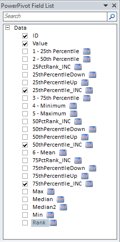
Figure 6 – PowerPivot Field List
Of all the measures shown, I want the client to see about half the number of measures in the list. The rest are intermediate results for development purposes only. To be honest, I don’t know which I find more baffling; that the development team can’t see the absolute necessity of this feature, or that I seem to be the only being on the planet that has a problem with this issue. Grrr. Unlike some very brilliant folks, I am unable to construct a half-page worth of a complex DAX formula, without the need to validate intermediate results.
On this matter, I think that I’m in good company. Flipping through the second edition of “The Microsoft Data Warehouse Toolkit,” written by authors from the highly regarded Kimball Group, I came across the following statement:
“The best way to create calculations and measures in PowerPivot is to break long, complex formulas up into their component parts and build them incrementally. This allows you to experiment with the data and quickly see the results of your formulas.“
Great advice, but incredibly, they don’t address how you are supposed to keep all of those intermediate results from the client’s view. The only solution currently available, and it’s a poor one from a performance and maintenance standpoint, is to merge the intermediate formulas into one mega-formula. Using perspectives don’t help either, since you can’t hide the original list of measures.
Rant #2
I’m glad to see that Denali includes TOPN, as this is a very useful function. But where is TOPNPERCENT? Can you name a product where these two functions don’t appear together, like Gemini or Siamese twins? Excel conditional formatting? Both there. Microsoft Access? Both there. T-SQL? Both there. MDX? Ditto. I find this level of inconsistency irritating. You can create a TOPN percent measure by using a formula like TOPN(COUNTROWS(Data)*N%), which is understandably trivial. Well, you can create a distinct count measure by using COUNT(DISTINCT), which is also trivial, but we now have DISTINCTCOUNT because creating distinct count measures are so common (and because the BI Pros all requested it J).
On the positive side, there is the “issue” of TOPN returning more than N records if there are ties in the Nth record. Microsoft’s products are somewhat varied in behavior. PowerPivot, Excel Conditional Formatting, and Access always return more than N values if there is a tie in the Nth value. MDX in Analysis Services never returns more than N values, so if there are ties in N, values are arbitrarily dropped (in contrast, SAS Analytics provides an option in MDX TopCount/BottomCount, which allows you to specify whether or not to return ties in N). T-SQL’s TOP predicate provides a WITH TIES qualifier to give you control over returning ties in value N. Personally, I see no logic in dropping tied values in the Nth record. Which records do you drop, and which record do you keep? Also, if there are ties in any of the values within the top N, all the ties are returned. Therefore, I think that PowerPivot, Excel and Access provide the correct logic.
Next…
In Part II, I will continue the discussion of percentiles using a slightly more complex example and demonstrate how to use percentile measures to create a box & whisker PivotChart!
